Essential Trig-Based Physics Study Guide Workbook Electricity and Magnetism

Essential Trig-Based Physics Study Guide Workbook Electricity and Magnetism

Pages: 491

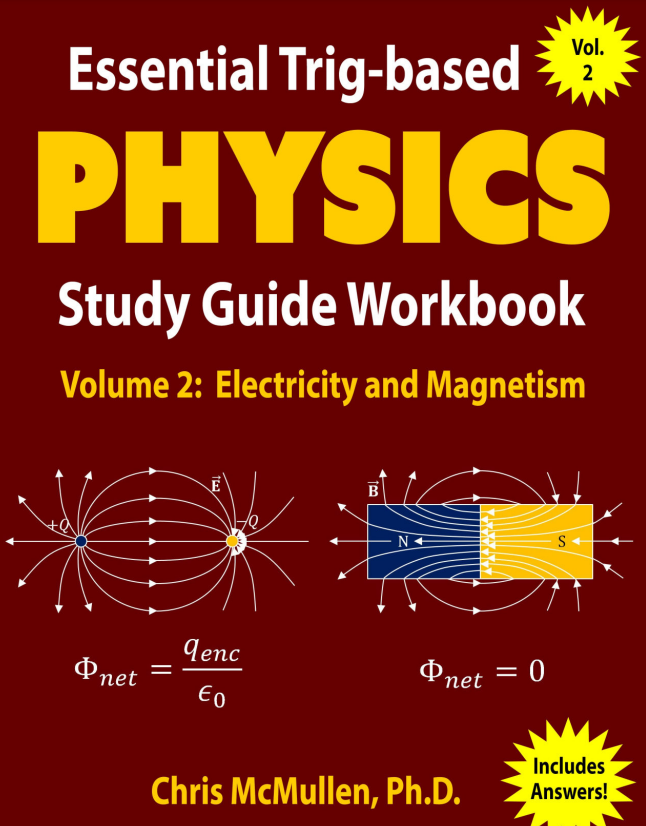
Essential Trig-Based Physics Study Guide Workbook: Electricity and Magnetism

Physics, the fundamental science, offers insights into the natural laws governing the universe. Electricity and magnetism, integral branches of physics, explore the behavior of electric charges, electric and magnetic fields, and their interactions. A firm understanding of trigonometry is essential for tackling problems in electricity and magnetism, as it underpins many concepts, calculations, and vector manipulations in these areas.

This guide serves as a comprehensive resource for students learning electricity and magnetism, with a focus on applications, formulas, trigonometric principles, and problem-solving techniques.

1. Introduction to Electricity and Magnetism

1.1 The Significance of Electricity and Magnetism

Electricity and magnetism are two interconnected phenomena that form the foundation of electromagnetism. Applications range from powering homes to enabling wireless communication and medical imaging.

1.2 Historical Background

The study of electricity and magnetism dates back to ancient Greece, with significant contributions from scientists such as:

• Charles-Augustin de Coulomb (Coulomb’s Law)
• Michael Faraday (Electromagnetic induction)
• James Clerk Maxwell (Maxwell’s equations)

1.3 The Role of Trigonometry

Trigonometry helps describe the spatial relationships between charges, fields, and forces. For example:

• Resolving vector components.
• Calculating angles between electric or magnetic field lines and forces.

2. Key Concepts in Electricity

2.1 Electric Charge

• Definition: A fundamental property of matter that causes it to experience a force in an electric field.
• Types: Positive (+) and negative (-).
• Unit: Coulomb (C).
• Trigonometric Relevance: In systems with multiple charges, angles and distances determine resultant forces and field strengths.

2.2 Coulomb’s Law

• Formula: F=k∣q1q2∣r2F = k \frac{|q_1 q_2|}{r^2} Where:
  • FF = Force between two charges.
  • kk = Coulomb’s constant (8.99×109 Nm2/C28.99 \times 10^9 \, \text{Nm}^2/\text{C}^2).
  • q1,q2q_1, q_2 = Charges.
  • rr = Distance between charges.
• Trigonometric Application: When multiple charges are involved, resolve forces using components: Fx=Fcos⁡θ,Fy=Fsin⁡θF_x = F \cos\theta, \quad F_y = F \sin\theta

2.3 Electric Field (EE)

• Definition: A region around a charge where another charge experiences a force.
• Formula: E=Fq=kQr2E = \frac{F}{q} = k \frac{Q}{r^2} Where QQ is the source charge.
• Visualization:
  • Field lines radiate outward for positive charges and inward for negative charges.
  • Angle calculations help map field vectors in multi-charge systems.

2.4 Electric Potential Energy

• Formula: U=kq1q2rU = k \frac{q_1 q_2}{r}
• Electric Potential (VV): V=Uq=kQrV = \frac{U}{q} = k \frac{Q}{r}

3. Key Concepts in Magnetism

3.1 Magnetic Fields

• Definition: A field created by moving charges or magnetic materials.
• Representation:
  • Symbol: BB
  • Unit: Tesla (TT).
• Trigonometric Application: The angle between the velocity of a charged particle and the magnetic field affects the magnetic force.

3.2 Magnetic Force

• Formula: F=qvBsin⁡θF = qvB \sin\theta Where:
  • qq = Charge.
  • vv = Velocity of the charge.
  • BB = Magnetic field strength.
  • θ\theta = Angle between velocity and field.
• Right-Hand Rule: Used to determine the direction of magnetic force:
  • Thumb: Velocity (vv).
  • Fingers: Magnetic field (BB).
  • Palm: Force (FF).

3.3 Biot-Savart Law

• Formula: dB=μ04πI dl sin⁡θr2dB = \frac{\mu_0}{4\pi} \frac{I \, dl \, \sin\theta}{r^2} Where:
  • dBdB = Magnetic field contribution by a small current element.
  • II = Current.
  • dldl = Length of current element.
  • μ0\mu_0 = Permeability of free space.

3.4 Ampere’s Law

• Integral Form: ∮B⋅dl=μ0Ienc\oint B \cdot dl = \mu_0 I_{\text{enc}}

4. Electromagnetism and Maxwell’s Equations

4.1 Maxwell’s Equations

1. Gauss’s Law (Electric Fields): ∮E⋅dA=Qencϵ0\oint E \cdot dA = \frac{Q_{\text{enc}}}{\epsilon_0}
2. Gauss’s Law (Magnetic Fields): ∮B⋅dA=0\oint B \cdot dA = 0
3. Faraday’s Law of Induction: ∮E⋅dl=−dΦBdt\oint E \cdot dl = -\frac{d\Phi_B}{dt}
4. Ampere-Maxwell Law: ∮B⋅dl=μ0ϵ0dΦEdt+μ0I\oint B \cdot dl = \mu_0 \epsilon_0 \frac{d\Phi_E}{dt} + \mu_0 I

5. Solving Problems Using Trigonometry

5.1 Vector Components

When dealing with forces, fields, or potentials, resolve vectors into components: Fx=Fcos⁡θ,Fy=Fsin⁡θF_x = F \cos\theta, \quad F_y = F \sin\theta

5.2 Angular Relationships

In rotating systems, angular velocity (ω\omega) and angular displacement (θ\theta) are crucial: v=rω,θ=ωtv = r\omega, \quad \theta = \omega t

5.3 Wave and Oscillation Analysis

• Electric and magnetic fields in electromagnetic waves are perpendicular.
• Trigonometric functions describe oscillations: E(t)=E0cos⁡(ωt+ϕ)E(t) = E_0 \cos(\omega t + \phi)

6. MATLAB® Applications

6.1 Simulating Electric Fields

x = -5:0.1:5;
y = -5:0.1:5;
[X, Y] = meshgrid(x, y);
Q = 1; % Charge
k = 9e9; % Coulomb's constant
r = sqrt(X.^2 + Y.^2);
E = k * Q ./ r.^2;
quiver(X, Y, X./r, Y./r);
title('Electric Field of a Point Charge');

6.2 Visualizing Magnetic Fields

theta = linspace(0, 2*pi, 100);
x = cos(theta);
y = sin(theta);
quiver(x, y, -y, x);
title('Magnetic Field Around a Current-Carrying Wire');

6.3 Solving Circuit Equations

Simulate Kirchhoff’s voltage and current laws for circuits:

R = [10, 20]; % Resistances
V = [10; 5]; % Voltages
I = inv(diag(R)) * V; % Solve for currents
disp(I);

7. Practical Applications

7.1 Circuit Design

Understanding charge flow and energy storage is key in designing capacitors and inductors.

7.2 Wireless Communication

Magnetic and electric fields are essential for transmitting electromagnetic waves.

7.3 Power Systems

Calculate energy loss and optimize efficiency using trigonometric techniques in power transmission.

8. Challenges and Tips

1. Handling Complex Numbers: Many problems in AC circuits involve complex impedance, which uses trigonometric identities.
2. Dimensional Analysis: Verify calculations by checking consistency in units.
3. MATLAB® Debugging: Ensure code accuracy by testing small segments before full simulations.

9. Conclusion

Electricity and magnetism are essential components of physics, enriched by the application of trigonometry and computational tools like MATLAB®. By mastering these principles, students and professionals can solve complex problems, innovate in technology, and contribute to advancements in engineering and science. This study guide offers a structured approach to understanding and applying key concepts, ensuring readiness for academic and practical challenges in the field.

Contents:

Chapter 1 – Coulomb’s Law 7

Chapter 2 – Electric Field 15

Chapter 3 – Superposition of Electric Fields 23

Chapter 4 – Electric Field Mapping 41

Chapter 5 – Electrostatic Equilibrium 55

Chapter 6 – Gauss’s Law 65

Chapter 7 – Electric Potential 89

Chapter 8 – Motion of a Charged Particle in a Uniform Electric Field 93

Chapter 9 – Equivalent Capacitance 99

Chapter 10 – Parallel-plate Capacitors 113

Chapter 11 – Equivalent Resistance 119

Chapter 12 – Circuits with Symmetry 133

Chapter 13 – Kirchhoff’s Rules 143

Chapter 14 – More Resistance Equations 155

Chapter 15 – Logarithms and Exponentials 165

Chapter 16 – RC Circuits